BLISS logo

BLISS: A Dataset and Benchmark for the Buckling of Imperfect Spherical Shells

Anonymous authors · under double-blind review

Does a surrogate that is accurate within distribution see the change when two defects start to interact?

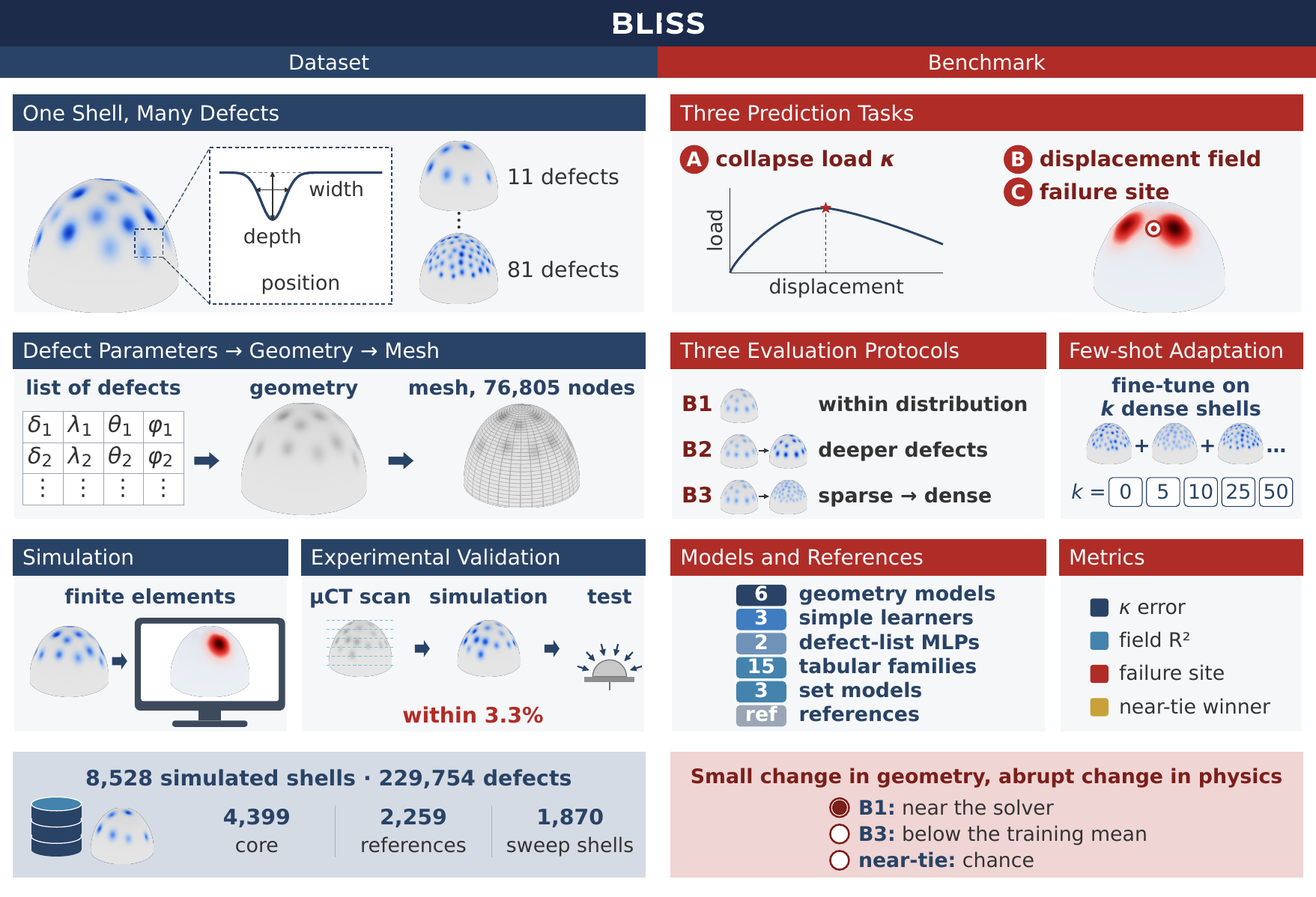
BLISS overview: dataset, simulation, protocols, models and metrics

Paper Highlights

8,528

shells simulated until collapse

0.985

buckling R² of the best model within distribution (B1)

B3 < mean

from sparse to dense, every geometry model scores below predicting the average training shell

−14%

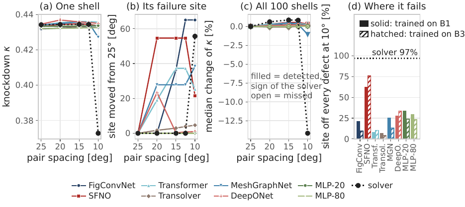
load drop when one pair moves 25° → 10°; models see ~0%

46–52%

near-tie decision after few-shot adaptation, where chance is 50%

Abstract

Machine-learning surrogates are increasingly used to predict how a structure responds to its geometry. However, existing scientific-ML benchmarks rarely use a change in the physical mechanism itself as the source of a distribution shift. Their shifts come from random splits, new initial conditions or held-out ranges of sampled inputs. Here, we introduce BLISS, a dataset and benchmark of 8,528 imperfect hemispherical shells simulated with finite elements until collapse, in which an instability creates the shift. A small change in geometry, two defects moving close enough to interact, changes how the shell collapses. Models map the surface with its defects to three outputs of the collapse, the collapse load (knockdown factor), the displacement field and the failure site where collapse starts. Within distribution, as on existing benchmarks, the best models reach a field R² of 0.985 and find 98% of clear failure sites. With deeper defects they lose the failure site where defects interact. Trained on shells with far-apart defects and tested on shells with close defects, every model that reads the shell geometry scores below a constant prediction of the average training shell on the field. Moving a single pair of defects from 25° to 10° apart lowers the collapse load by 14% in the solver, while the models predict almost no change. Five dense examples recover most of the field of two models, and the choice between two nearly equal failure sites stays close to chance. Our simulations match eight physical tests within 3.3%.
Dataset

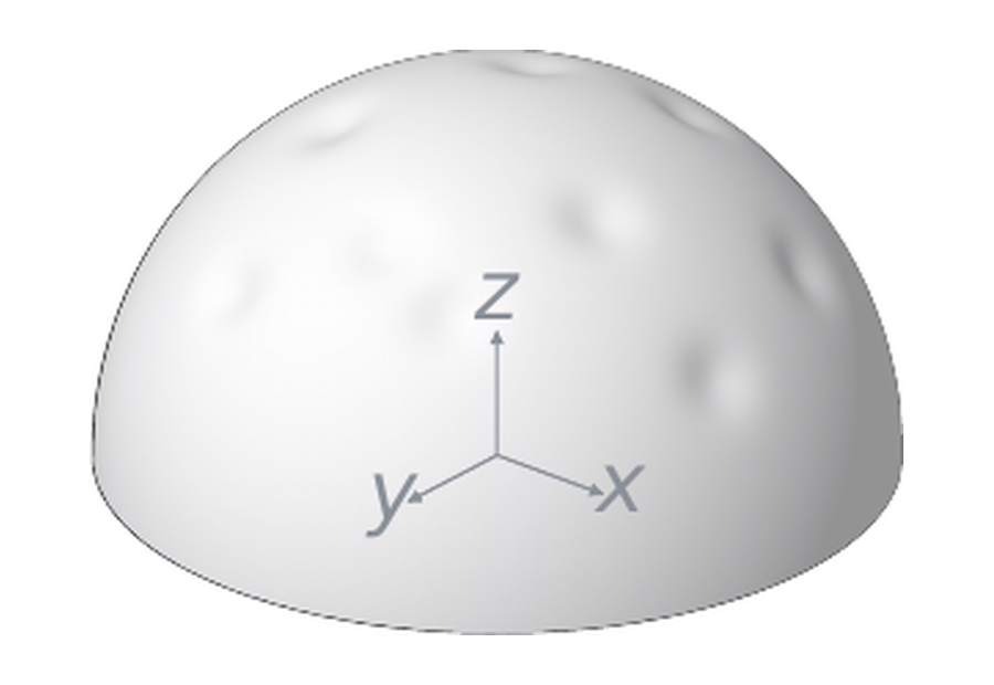
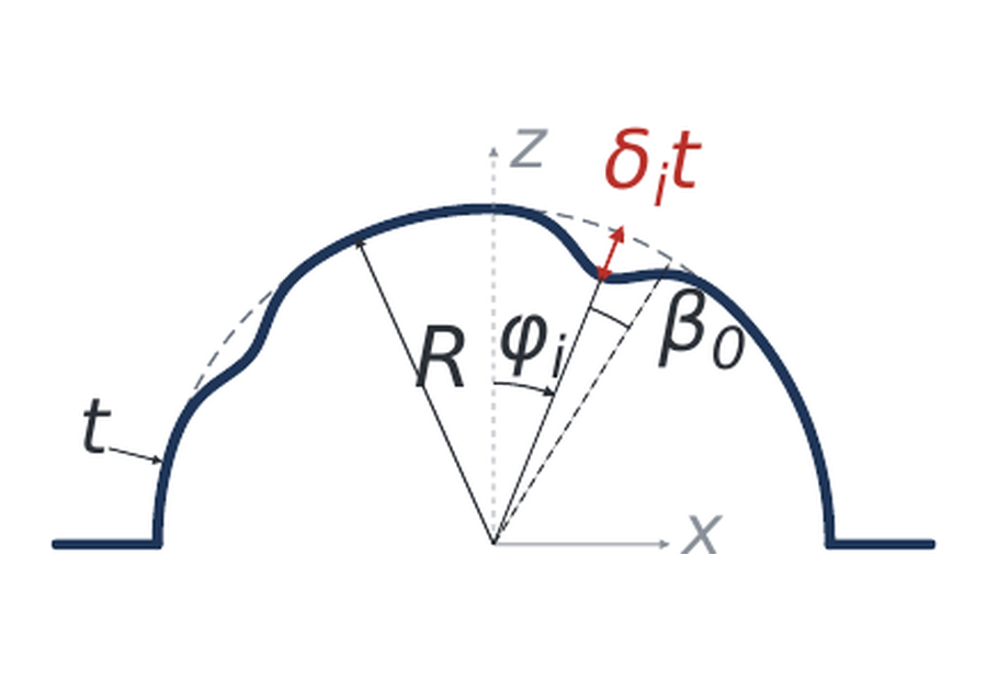
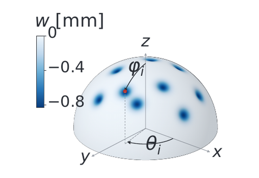
Thin shells, such as pressure vessels and launch vehicles, collapse by an instability, and a defect as deep as the wall thickness can halve the pressure a shell carries. When the defects of a shell are far apart (sparse), each acts alone. When two come close (dense), they buckle as one region and weaken the shell differently. Each BLISS sample is one clamped hemisphere (R = 25.4 mm, R/t = 110) with small inward defects, loaded by external pressure and solved with nonlinear finite elements until it collapses.

imperfect shell
(a) an imperfect shell
one defect
(b) one defect: depth, width, position
surface deviation w
(c) the input w at every node
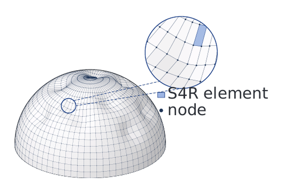
mesh
(d) the shared mesh, 76,805 nodes

What is released

blockshellscontent
core4,39911 to 81 defects; w, displacement at the peak and one solver step on either side, load path, κ, site ratio q
intervention tests P1–P41,870core shells edited one factor at a time (rotate, move, bring closer, delete defects), same fields, with their source id; evaluation only
single- and two-defect shells2,259defect parameters and κ as table rows
total8,528all simulated by the authors; checked by a mesh study and against eight physical tests (within 3.3%)

Files

filecontent
shared.npzthe shared mesh: unit node directions P (76,805 × 3), S4R connectivity conn, radius R, and the map to the 180 × 720 grid
canonical/<id>.npzone record per core shell: w (input), kappa and U_peak (targets), U_prev, U_next, mode, the load path lpf with peak_frame, and q, r_d2_d1, implied_gap_pct
sweeps/the records of the intervention tests P1–P4, same keys, with the id of their source shell
metadata/one row per shell (shells.csv) and per defect (defect_parameters.csv: δ, λ, θ, φ), the site ratio q and the two competing sites (truth_dominance.csv), and the single- and two-defect shells
splits/B1.json, B2.json, B3.json: the three protocols, fixed with seed 2027

Terms used on this page

  • Knockdown factor κ: collapse pressure over the classical pressure of the same shell without defects.
  • Sparse / dense: any two defect centres at least 25° apart (11 to 18 defects), or at least 10° apart (69 to 81 defects).
  • Failure site: where the buckling deviation (the displacement after removing the uniform contraction) is largest.
  • Site ratio q: amplitude of the second competing site over the first. Clear winner: q < 0.7. Near-tie: q > 0.9.

Dataset Explorer

The shells of the review subset that carry the full simulation. Pick a family, then a shell in the list or in the parameter plot. The shell is drawn from its list of defects with the generator of the dataset; switch to the shape at collapse and after it, and follow the load path of the simulation.

The family in its parameter space; the selected shell is outlined. Click a point to open it.

Click a row to open the shell.

Load the Data

One command of the code repository downloads the review sample. Every shell is one .npz file on the shared mesh, so it is read with NumPy alone, and the bliss package adds the three protocols and the scorer.

# download the review sample (290 MB) into BLISS-1.0/, check its SHA-256 and link it for the scripts
python benchmark/data/download.py
# one shell with NumPy
import numpy as np

mesh = np.load("BLISS-1.0/shared.npz")
P, conn = mesh["P"], mesh["conn"]  # nodes, elements
s = np.load("BLISS-1.0/canonical/2384.npz")
w = s["w"]         # (76805,) input
U = s["U_peak"]    # (76805, 3) target
s["kappa"], s["q"], s["lpf"]  # κ, site ratio, load path
# with the benchmark loader
import bliss
from bliss.metrics import score_ci

d = bliss.load("BLISS-1.0")
train, val, test = d.split("B1")  # or "B2", "B3"
s = d[test[0]]
s.w, s.U, s.kappa                 # input, targets
s.defects                         # (n, 4) defects
score_ci("preds.npz")["metrics"]  # all metrics

Install and the commands that reproduce every result are in the README of the code.

Benchmark Protocol

From the surface deviation w, predict κ, the displacement field at the peak load and the failure site. Six geometry models read w on 8,192 nodes (SFNO on its 180×720 grid), and three simple learners (nearest neighbour, PCA-ridge, gradient boosting) read w too; twenty models read the list of defects instead (15 tabular families, three set models, two MLPs); references need no training. Three controls retrain models on the full mesh (76,805 nodes), on 2,048 nodes and, for SFNO, on a 64×128 grid. Every learned model is the mean of three seeds, with hyperparameters searched on B1 and frozen for B2 and B3.

protocoltrain / val / testwhat the model has seen, and what it is asked
B1 within distribution3,299 / 440 / 660random split (seed 2027): test shells like the training shells, the role of existing benchmarks
B2 deeper defects2,789 / 376 / 1,234test shells have their deepest defect above 2.35 t, deeper than in training
B3 sparse to dense1,934 / 265 / 2,200trained only on far-apart defects, tested on close defects that interact: the shift the instability creates
  • MRE κ: median relative error of the knockdown factor.
  • Buckling R²: R² of the displacement field after removing each shell's uniform contraction.
  • Clear-site accuracy: share of clear winners whose predicted site lies within 10° of the true one.
  • Near-tie winner rate: on near-ties, share where the model deflects more at the true site than at the second candidate (chance 50%).

Leaderboard

Table 2 of the paper. Learned models give the mean over three seeds; field metrics after removing the uniform shrink; bold red marks the best learned model on 8,192 nodes. Click a column header to sort. † reads the list of defects. ∗ SFNO on a 64×128 grid. ‡ deepest point of w. div.: diverged. Full-mesh B2 and B3 are reported for FigConvNet, SFNO and Transolver. Models differ in input (w or the list of defects) and output (field and κ, or κ only): the table lists every model that predicts the field and the best κ-only model, and the other models are in the full tables below.

Ranking

Every model and reference of the selected protocol, best on top, with the 95% shell-bootstrap interval. Click a bar to open the model.

Show all models and all metrics (the full results tables of the paper)

Headline columns carry the 95% shell-bootstrap interval; the regime columns split the test set into its sparse and dense shells (B3 tests on dense shells only).

Results

B1 → B2 → B3 · three protocols

Within distribution every model looks good; from sparse to dense they all lose to the mean

On B1, the split that plays the role of existing benchmarks, FigConvNet, MeshGraphNet and the Transformer reach a buckling R² between 0.968 and 0.985, while the solver states one step before and after the peak reach 0.993 and 0.966. With deeper defects (B2) the best models keep the field and lose the failure site on dense shells. From sparse to dense (B3), every geometry model scores below the training mean on the field, with a buckling R² from −1.31 to 0.29 against 0.340. The ranking inverts: FigConvNet is the best on B1 (0.985) and the worst on B3 (−1.31).

One line = one model, the mean over three seeds; dashed grey = the training mean. Click a chip to hide a model.

Accuracy within distribution does not predict accuracy under a shift created by the physics.

B1 vs B3 · the same shell

The same dense shell, two training sets: the site is found, then lost

Each model predicts the same dense shell twice: trained on B1 (dense shells seen in training) and trained on B3 (sparse shells only). Look at the crosses first: they mark where the solver says collapse starts. A circle on the cross means the model found the failure site. On sparse shells collapse starts at the deepest defect (all 94 sparse B1 test shells with a clear winner), so models trained only on sparse shells put collapse there; on dense shells this holds on only 38% of the clear winners.

Seed-0 models of the paper, scored on the 8,192 nodes, seen from the pole. Colour: magnitude of the buckling deviation. Percentage: error of the predicted κ.

Models trained on non-interacting defects extrapolate that response to shells where it no longer holds.

P3 · intervention test

One pair moves from 25° to 10°: the load drops 14%, the models see almost nothing

In 100 sparse B1 test shells one pair of defects is moved from 25° to 10° apart and every other defect is kept. The median drop of κ at 10° is 14%, and the failure site leaves every defect on 97% of the shells. The B1-trained models predict median changes between −1.1% and +0.3%, and none recovers half of the true drop on more than 3% of the shells.

Intervention test P3

The B1 models saw dense shells and still respond to one close pair as to a sparse shell.

Few-shot · B3

Five dense shells repair the field, not the near-tie decision

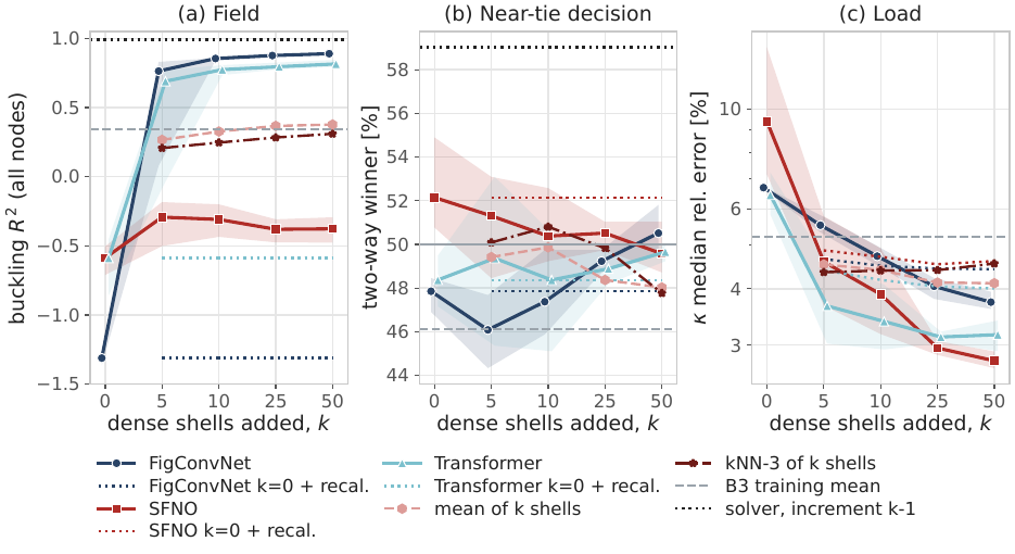
With five dense shells FigConvNet and the Transformer reach a buckling R² of 0.76 and 0.69, up from −1.31 and −0.59, and 0.89 and 0.82 with fifty. The near-tie winner rate stays between 46% and 52% at every k.

Few-shot adaptation

Choosing between two nearly equal failure sites remains an open problem.

Scope and Future Work

By holding the shell family and load case fixed, BLISS is designed to isolate geometry-induced changes in the instability mechanism, so that changes in model performance can be attributed more directly to geometry. Extending this controlled setting to other structures and loads, and learning the near-tie decision, are the next steps.

Resources

  • Data: the review subset on OSF (link above); the full release of 8,528 shells is available to reviewers on request and will be public at publication, under CC BY 4.0.
  • Code: the loader, the scorer, the eight field models with one training recipe, the search, the models on the list of defects, the references, the intervention tests, the results tables, the three split files and a script that downloads the review subset, under MIT (anonymized repository).

Citation

@misc{anonymous2026bliss,
  title  = {BLISS: A Dataset and Benchmark for the Buckling of Imperfect Spherical Shells},
  author = {Anonymous},
  year   = {2026}
}